Would you like to understand why many reported immunoprecipitations and pulldowns are unreliable? Are you worried that your immunoprecipitations, pulldowns, or affinity purifications aren’t as compelling or as efficient as they could be? Then read on.

Immunoprecipitations (IPs), GST pulldowns, affinity purifications, pelleting assays, and classical biochemical fractionation of cytosol & organelles – they all involve the physical separation of a mixture into two or more parts (fractions).

And fractionation, as an analytical technique, is how to quantitatively analyse that separation process. It lets you know how much of your target protein you’ve immunoprecipitated or pulled down, how much of the binding partner has come down with it, what the yield in your purification was like, and whether different pools of a protein exist within a cell.

And it’s easy. Much, much simpler than people suppose.

To explain how to use it properly, we’ll use both hypothetical and real-world examples, and illustrate some common pitfalls.

Example 1:
Here we have an input mixture (I) being separated by centrifugation into two fractions: a supernatant (SN) and a pellet (P). It’s important to stress again that the separation can be any physical process, not just centrifugation – you could have bound/unbound fractions instead, for example.

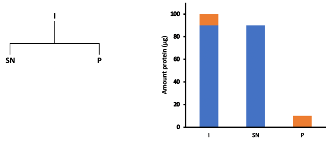
In this example, let’s assume that the input contains 100 μg of protein, of which 10 μg is our protein of interest, and the other 90 μg is other stuff. If our centrifugation achieves perfect separation then the 90 μg we’re not interested in goes into the supernatant, while all 10 μg of our target protein goes into the pellet.

To analyse this process, we need to take samples of each of those fractions, let’s say 1%. In practical terms, this would mean taking a 1% sample of the input before the centrifugation step, taking a 1% sample of the supernatant after the centrifugation, and then resuspending the pellet in a new solution and taking a 1% sample of that. Don’t neglect to take that input sample! You’ll see why in a moment.

We then load equal fractions on a gel, and for simplicity let’s say we load the whole 1% of each fraction. The equal fraction is the critical thing – it could be 1%, 0.5%, 0.1%, whatever, so long as it is the same, and for all fractions. We then visualise the protein of interest (POI) by immunoblotting.

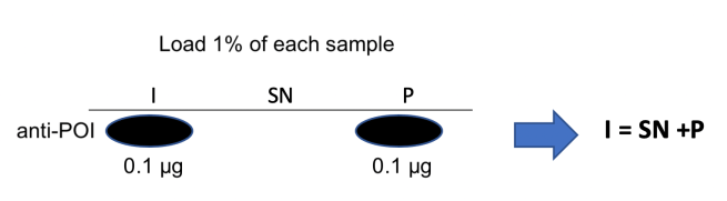
Our Input mixture was 100 μg, so the 1% sample is 1 μg, of which 0.1 μg is the protein of interest.
Our supernatant was 90 μg, so the 1% sample is 0.9 μg, none of which is the protein of interest.
Our pellet sample was 10 μg, so the 1% sample is 0.1 μg, all of which is the protein of interest.

Consequently, we find that I = SN + P. This tells us that we have accounted for all our protein, and that it has wholly partitioned into the pellet fraction. This is also why it is critically important to take an input sample, because that tells you what the total amount of material is. If I > SN + P, that immediately tells us that we have had losses during the procedure. And if our protein is present in both the SN and P fractions, we’ll be able to say what the proportions are.

The beauty of this is that while we’re using μg protein here, we could just as easily be using sample volumes. If you started off with 1 ml of your mixture, and got 900 μl SN and 100 μl of resuspended pellet, you’d be loading 10 μl, 9 μl, 1 μl for your 1% samples, and you’d get the same result. In fact, you could even resuspend your pellet to a total volume of 1 ml, take a 1% sample of that (10 μl), and you’d still get the same result. As long as you always load the same % fraction of each sample, you’ll get accurate information on how things are partitioning (crunch the numbers if you’re unsure).

 

Example 2:
Here’s a real-world example of a one-step fractionation, with the Input (I) – a cell lysate produced by detergent extraction – separated into cytoplasmic supernatant (SN) and cytoskeletal pellet (P) fractions. Equal fractions have been loaded in each lane. Note how I = SN + P. In other words, every protein band in SN and P adds up to its counterpart in I.

 

Example 3:
Now let’s consider a more complex example. Here’s a two-step fractionation scheme, where the P1 fraction has been further fractionated into SN2 and P2 fractions.

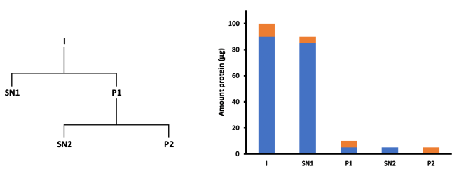
As before, let’s assume that there is 100 μg in the initial input, 10 μg of which is our protein of interest.
This time, we get 90 μg in SN1, of which, say, 5 μg is our protein of interest, and 85 μg is the other stuff.
P1 is therefore 10 μg, made up of 5 μg of our protein of interest, and 5 μg other stuff.
If the second fractionation step perfectly separates the P1 fraction, then the 5 μg of other material goes into SN2, and the 5 μg of our target protein ends up in the final pellet (P2).
Also, as before, let’s assume that we take a 1% sample of each of the 5 fractions, and load the whole 1% on a gel before immunoblotting for our protein of interest. Here’s what the blot will look like:

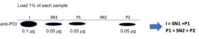
The input sample was 100 μg, so our 1% sample is 1 μg, of which 0.1 μg is our protein of interest.
The SN1 sample was 90 μg, so our 1% sample is 0.9 μg. There were 5 μg of our protein of interest in SN1, which means there is 0.05 μg in our 1% sample.
The P1 sample was 10 μg, so our 1% sample is 0.1 μg. 5 μg of P1 was our protein of interest, so there is 0.05 μg of it in our 1% sample.
The SN2 sample was 5 μg, so our 1% sample is 0.05μg, none of which is our protein of interest.
The P2 sample was 5 μg, so our 1% sample is 0.05 μg, all of which is our protein of interest.

Now we really see how powerful fractionation is for tracking the partitioning of objects of interest.
I = SN1 + P1, which tells us that we have accounted for all of our protein. As the band intensities in SN1 and P1 are the same, that tells us that the protein is partitioning evenly between the two fractions. If this was a purification, that would tell us that the yield for this step could be improved (centrifuge harder or longer perhaps, or add more antibody in an IP); if this was cellular fractionation, it might suggest that there are distinct biochemical pools of the protein (e.g. cytosolic and cytoskeleton-associated).

Furthermore, P1 = SN2 + P2, which tells us again that we have accounted for all of our protein. And because P1 = P2, we know that the protein has wholly partitioned into the second pellet fraction.
Let’s take a look at another, more complex, real-world example…

 

Example 4:
This is an expanded view of the same experiment used in example 2, which was actually a proximity-dependent biotin identification (BioID) experiment. After the first extraction step, the cytoskeleton pellet (P1) was further extracted in 0.4% SDS, a sample taken, and the solubilised material (S2) separated from the insoluble material (P2) by centrifugation. The cytoskeletal (S2) fraction was then incubated with streptavidin-coated magnetic beads to bind biotinylated candidates and separated using magnetic beads into unbound (“free”, S3) and bound (P3) fractions.

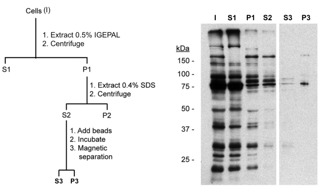
Equal fractions were loaded on the gel, and blotted using a streptavidin conjugate to detect biotinylated proteins.
I = S1 + P1, which tells us that we have accounted for all biotinylated proteins in the first fractionation step.
P1 ~ S2, which tells us that there have not been significant losses during the second extraction step (in other words, SDS has extracted almost all the protein in P1; P2 not shown).
S2 >> S3 + P3, where P3 is the material bound to the beads. This presents a puzzle. The near absence of material in S3 suggests that all of the material in S2 was captured by the beads, but the bound fraction, P3, appears to have very little protein. This tells us that there is unaccounted material – and indeed, this proved to be the case. The streptavidin beads were binding the biotinylated protein so tightly that there was not significant elution even after boiling in SDS loading buffer (!) As a result, the proteins had to be trypsinised on the beads and analysed directly using mass spectrometry. Correct use of fractionation allowed optimal detection of the captured proteins.

Lastly, let’s consider some common pitfalls in the reporting of fractionation results, specifically those relating to immunoprecipitations (IPs) and pulldowns.

 

Example 5:
Immunoprecipitations (IPs) and GST-pulldowns are two key biochemical techniques in molecular cell biology, but they are seldom correctly reported. In an IP, an antibody is used to pull down a target protein, after which co-immunoprecipitating proteins can be analysed; in a GST-pulldown, the target protein is expressed with a GST tag and itself used to pull down interaction partners. There are many variations – the antibody or GST-protein can be immobilised on beads either before or after the binding step, the mixture probed can be a cell lysate or a defined combination of recombinant proteins, and so on – but they all share the same basic scheme: you have an input mixture which is separated into an unbound/flow-through fraction and a bound/IP fraction (see below).

Unfortunately, it’s not unusual to see such experiments reported in the style shown on the right, in which the interaction between a dynein motor adaptor (BICD1) and a protein tyrosine phosphatase (PTPN23) is being probed. The protein BICD1 has been immunoprecipitated and the IP fraction has been immunoblotted (IB) to see if PTPN23 has bound and co-immunoprecipitated. A non-binding antibody (rabbit IgG) has been used as a negative control condition (it’s worth noting that this is a much stronger negative control than a simple no-antibody reaction, because it means that proteins non-specifically interacting with rabbit IgGs can be excluded with confidence).

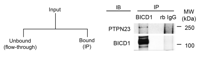
See the problem? This is a one-step protocol, but we’re only being shown the IP – neither the input sample nor the unbound fraction has been disclosed! This tells us very little. We have no idea how much material there was to start with (because there’s no input shown), how much of the BICD1was immunoprecipitated, or how much of the PTPN23 came with it (because there’s no unbound fraction shown). All we know is that when the bound fractions were blotted, both proteins could be detected. But what if the PTPN23 that co-immunoprecipitated was only 0.01% of the total? Would this really represent an authentic interaction? The reliability of the result is almost impossible for a reader to assess, because so little information has been provided.

A slight improvement is to report the results as follows:

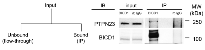
This initially seems better, because there’s disclosure of both the input and the bound samples, but do you see what the problem is now?

Here, the unbound/flow-through has still not been reported, and although an input sample is shown, there’s no disclosure as to whether equal fractions have been loaded. All we know is that both proteins were present in the input and the IP samples, but we have no sense of the relative amounts in the different fractions. Once again, and despite first impressions, we have no idea what the yield in this protocol is, and consequently cannot be sure of the reliability of the interaction.

Now let’s look at the blot, as it was actually shown in Fig 1A of Budzinska et al., 2020 (some extra annotation provided for clarity).

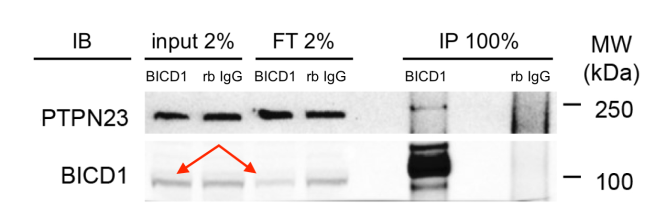
Here, both input and unbound/flowthrough (FT) samples are shown alongside the IP, so all three fractions are reported.
The input and FT fractions are shown at 2% (disclosure is in the M&M, and added to the image here for clarity), while the IP is shown at 100% – this explains the discrepancy in band intensity between the input and IP lanes, because a 50x greater fraction has been loaded.

Comparison of the input and FT lanes (red arrows) allows you to see the amount of the total BICD1 has actually been immunoprecipitated.

For PTPN23 there is essentially no difference at all between the input and FT lanes, though some can nonetheless be faintly detected in the IP for BICD1, perhaps around 0.2% of the input.

As the authors note, “Endogenous PTPN23 was consistently isolated in BICD1 immunoprecipitates (Fig. 1A), albeit at low abundance, suggesting that the association between these proteins may be transient, or alternatively, that only specific sub-pools of these two proteins interact in neuronal cells.” The IP is undoubtedly weak, as they concede, but it’s there, and because they’ve provided the reader with all the information necessary to interpret the experiment for themselves, that inspires confidence in the appropriately cautious conclusion (which, it should be noted, they go on to conclusively validate).

This is a great example of how the correct application of fractionation as an analytical technique allows a precise and higher-confidence statement to be made, even when the interaction is a weak or transient one.

Clear? Let us know if not.
Acknowledgements:
This posting co-authored with Graham Warren.
A big thanks to Giampietro Schiavo for letting us feature the IP from Budzinska et al.